Project page
Welcome to the deep learning project blog where a journal of the project's progress will be kept.
Before the project started
The first assignment was to implement an MLP. Since it was already done in the Machine Learning class last semester, I instead tried my hand for the first time at Theano and implemented an MLP with it.
Week of the 1st of February and 8th of February
I will concentrate my efforts on the Vocal Synthesis project. I familiarized myself with LSTM, installed blocks/fuel and started to try to understand how to use a simple LSTM for this task using blocks' framework.
Week of the 15th of February
Late update for that week as I was out of town for the weekend. This week I listened to Alex Graves' presentation on how to generate sample. I had trouble wrapping my head around everything. I will try to explain the basic idea of what I understand. First you have an RNN, on top of it you fit its output with a mixture of Gaussians from which you sample. These samples generate the next sequence. That's all good but what of the training process? How do you backpropagate a gradient to train the RNN? You could use the EM algorithm for the mixture phase, but then I don't quite understand how to train the RNN. An idea would be to do gradient descent on the likelihood as a cost function on the mixture of Gaussian, this would allow the gradient to go down the RNN. Okay, let's try to just do the mixture model.
First I thought of a model like this x -> h -> L <- x where x is the vector of input and h a shorthand for three independently computed quantities : m mixture coefficient, a averages of Gaussians and its s standard deviations, finally L the cost which is simply p(x ; m, a, s) = mixture of Gaussians (not sure I can type this equation on github) After asking around, I was told that this would not produce what I had hoped. It would instead learn a different distribution for every x. The good model would be to let m, a and s be free parameters like this : x -> L <- h. Not sure I understand why...
Week of the 22th of February
Implementation of the first model x -> h -> L <- x. It did not work as expected! However, this is the one that I think will be used on top of the RNN so its not wasted time.
After a lot of conversation with people knowledgeable in generative models, looks like this approach is not going to work and was a waste of time. I investigated the other idea of doing EM on the output of the RNN. It could work, the problem is that you don't have an analytical (meaning I failed at taking a paper and do the derivatives by hand) gradient on the EM part of the model and thus cannot train using backprop the RNN under it. The only thing that sounds promising at this stage is to try making the free parameters model on last week post work, however so far it just doesn't want to converge on the good distribution. This sounded so simple and elegant on Alex Graves' presentation, one small equation P(x_t|x_1:t)...
Week of the 29th of February
I finally decided to try the model (the very first idea) with an RNN that would take x_t and spit out x_t+1. Now in order to compute anything meaningful for training, I need to give a gradient to the RNN. So on top of that, I will have a mixture of gaussians computed with EM. This will allow me to a) sample from it in the generative process and b) compute the likelihood during training from this mixture with the true x_t+1. Someone reading this will feel like I have been circling around the same ideas for three weeks, which is not quite false but not quite true, let's try to wrap it up a little and make it clearer :
From Alex Graves' presentation I wanted to do this simple thing, a mixture of gaussian on top of an RNN. A choice arrived : how do you find the mixture? You can do gradient descent on the whole thing (RNN + GMM) or use something else like the EM algorithm for the GMM. The first solution would be the simplest as everything would live in Theano so I tried it first. This solution required me to understand the differences between the two models proposed on the Week of the 22th post. Then after much work, just the mixture model (x -> L <- h) never converged with the fake data. Even worst, it occurred to me that if it would failed to converge on the fake data which are infinite (you can generate simple mixtures with numpy) it would for sure fare poorly on the real task. So then I moved to the second solution. I was reluctant to do this one as it would require dealing with an algorithm inside Theano and outside Theano and there are still open questions such as : Do you fit a new GMM on each sequence produced by the RNN or do you refit it with the already learned parameters from the past fits as the EM algorithm is very sensible to initialization? Also, the fit is after the RNN and the gradient for the RNN is after the fit, so there is no joint training of the model, they are in kind of independent phase and I am not sure if that is a good thing. You can't do a common trick of training on one epoch the RNN with the GMM fixed and the other epoch find the GMM with fixed parameters on the RNN because in this context it makes no sense. If you fix the GMM during an epoch, the likelihood for the gradient are taken from this GMM with the true sequence x_t+1 so it does not depend on whatever state the RNN produces! Looks like I don't get the whole picture yet but I decided to go with it anyway and I dealt with the inside/outisde Theano problem which is explained on the next paragraph.
The challenge this week was to wrap my head around blocks and fuel. The problem is that the EM will be done by sklearn so outside Theano and the likelihood will be computed inside Theano. So first I tried to hack fuel by trying to pass the parameters of the mixtured as a DataStream channel, that didn't went far. Second I tried to find a way to give this to blocks, the reason is if I can work it out with blocks I will have access to all these already coded bricks like the LSTM. It took me a long time to understand but all I needed was the ComputationGraph class from which you can easily get the parameters of all your bricks. You can then build yourself a gradient and use theano.function with your own inputs and cost and boom magic. Handy trick to know.
I have implemented these ideas with a fake data and a brick MLP, I just wanted for this week to get the code executing without error so next week comes the real dataset.
Week of the 7th of March
This week was much about programming, I implemented and fixed bugs for the model of last week with the true LSTM brick. On a few test run the likelihood seemed to be going down. I also added a few monitoring stuff since it is going to run on a GPU now. Let's see if at least the likelihood is going down through some epochs and after that, generation time.
Unfortunately, at some point right before the change of epoch the likelihood suddenly goes to NaN. I have implemented a feature to save the model's parameters and spend most of my time debugging that.
Week of the 14th of March
The beginning of this week was characterized by again going back to previous ideas and redoing a lot of things. I was not able to debug the NaN in the rnn_em model.
However, this week was kind of a milestone for this project : I decided out of curiosity to go check the actual paper of Alex Graves' presentation and boom. I finally realized and understood what he meant by those mixtures of Gaussian and how to completely backpropagate on it using RNNs, no need to go out of Theano or mess with the nonsense of the EM... lesson : READ THE PAPER!
I went back to my code and programmed this new model named lstm_gmm. In other words, everything that was done in the pasts weeks are almost completely useless. Almost because I learned a lot on the model and the programming frameworks. What took me most of my time this week was that I had to figure out how to use all these Blocks' bricks and some numpy broadcasting magic but it all worked out. It is now running (10 times faster since it can stay in Theano) and will start generating sound. Now I might even be able to run everything with blocks and use the MainLoop class so I might sadly scrap what I did if I make the change.
Week of the 21st of March
The model now get stuck on one mixture by setting its probability to one and the others to zero. Doing so causes underflow on the GPU and makes it crash. I have now put a sigmoid before the softmax of the mixutres to prevent a spike on one mixture. I have also noticed it does crazy stuff on the averages of the Gaussians like setting one to -250 when the data is normalized between -1 and 1. To prevent that, I now have a 10*tanh before the averages so it is constrained between -10 and 10. I was able to not make the GPU crash with underflows with these additions but the likelihood got stuck very fast and it didn't train very well.
A few days later I implemented the logadd function like we learnt in the machine learning class. logadd(a, b) = m + log(exp(a-m) + exp(b-m) where m = max(a, b). It is now way more numerically stable and the likelihood dropped by a lot! Still, the same kind of behaviour persists. It seems that I either give the model not enough capacity so the likelihood just oscillates because of variance in the data, giving me false impression of training but actually nothing is trained. Or, I give it too much capacity and it settles very quickly into a region and doesn't move from there.
I see three explanations or ways to move forward here : First the right capacity for this learning task is in a very narrow region and would require extensive hyper-param tuning, second it could just not a good model for this task or third my code is simply bugged. I spent quite a lot of time this week on the first option and running different experiments with different values of the LSTM dimension or GMM with me always falling into one of the two cases mentioned earlier. Now to rule out the third option I would have to port this model to exactly reproduce the handwriting experiment in the original paper. I ought to try that, but time is slowly running short...
Week of the 28th of March
So this is going nowhere. I noticed a nasty bug but even by fixing that it keeps on having the same behaviour as explained last week. I could still technically implement the original paper and see if I am doing something wrong when computing the cost function, but it seems to me the failure is not there.
I have carried on with my motivation on why I tried this paper on the first place. I wanted to apply it on the frequency domain where it makes sense to model each frequency bin of the spectrogram as a Gaussian. The raw audio signal seems too messy to try to learn something sensible.
This week I restructured the code and implemented that idea on a new python script, but of course, on the first execution I was welcomed with NaNs. To be continued next week.
Week of the 4th of April
This week was intense! First I rewrote the two scripts, the one that works in the time domain and the other one for frequencies, so that they could use the MainLoop of blocks and also made the data handler to be in fuel. The reason behind this is that as I was mentioning in the past weeks, I think I ran into an optimization problem. That being said, I needed to use things such as AdaDelta, Momentum, etc, and they are all contained in blocks. I had to write my own class for a fuel scheme as no scheme supported overlapping in the operation process. By overlapping I mean a scheme that, for example, gives me 5 time points on the first batch so [0,1,2,3,4] and second batch [4,5,6,7,8] and so on, the overlap here being on the 4.
Even with all of that the training was going nowhere, I lost track of all the configurations (number of LSTM layers, LSTM dimension, time dimension,...) I tried, for all of them nothing was being learned.
Second big milestone : I went to talk to Alex Nguyen who was generating nice sounding samples and I realized one very stupid thing I was doing. He is generating sequences while I was trying to generate one time point : For example, my time dimension in my LSTM is half a second so 8000 and my input dimension is 1 for one time point. In what he is doing, his time dimension is now a sequence dimension of say 10, and his input dimension is now the time dimension of 8000 points!
Of course! Like I thought (and was trying to fix by going to frequency space), an audio signal is way too crazy one time point at a time, it makes way more sense to have a model that can generate a sequence (like one second which would be 16000 points) then trying to learn what it should do for just one tiny point. I went ahead with this, now my GMM would try to fit a distribution that gives t number of points and learn on s sequences. The mathematics would go like this :
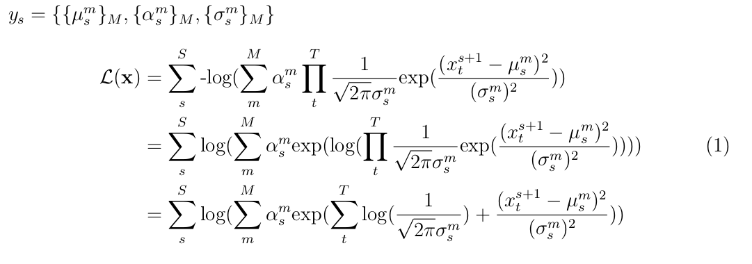
The first line is the output of the RNN, as it was being said, we interpret the output of the LSTM as a set of M mixtures of means, mixture coefficients and standard deviations. Since there is one such output for every sequence of t points, that's the s subscript. x is a matrix of sequences by time points. The equation details the likelihood that is implemented in the script (last line).
I have to thank Jose Sotelo and Kyle Kastner as I had a nice discussion with them to help me understand what was happening. After modifying my model for this cost function and having sequences, my first run was of course NaNs. After much failed trials, Jose again was of great help. As he trained GMM too, he gave me tricks like putting epsilon values everywhere there was a logarithm to prevent underflows and play around with the log(sum(exp)) math trick to make it numerically stable. For the first time in two months the likelihood was actually going down across multiple epochs, not randomly oscillating!!!!! I encountered an interesting problem though that it would crash to NaNs after a certain number of epochs while switching from the end of one to the next. So far, for every epoch I was sequentially passing through the whole soundtrack, I thought it was necessary to do this. Seems like my understanding of the LSTM was not complete, I thought that you needed to start the next batch to the same point where you ended the last one. That's not true, the LSTM can only learn the time structure over the dimension of time you give it, basically different set of sequences are independent of each other (this would seem very obvious but it wasn't). This means I can shuffle the data in chunks of sequence length and that fixed my problem mentioned above, looks like it was overfitting and got crazy with the transitions from the end of the song to the beginning when going to a new epoch.
I implemented a fuel scheme that would shuffled the whole data set in chunks of sequence length and a fuel transformer that reshaped my data (to be noted that this meant the first overlapping scheme programmed this week is now useless). The learning algorithm is also optimized with Adam. Now it is learning past an arbitrary amount of epochs. I am still exploring the set of parameters that gives the lowest likelihood and shall generate something next week. Will it finally sound like something?
It is to be noted here that the state of my script is now more close to the original paper. There are no sigmoid before the softmax or tanh or whatnot like it was mentioned on the Week of the 21st of March
Week of the 11th of April (including the 18th)
At the beginning of the week, the new setup with sequences of time points made me realized that my ambition of playing around in the Fourier space was iced down. On a usual example of ten sequences of 16000 time points, going for these 10 sequences and mapping all these time points in the frequency domain would have expanded to way too many datapoints to fit in the GPU. I abandoned maintaining lstm_fourier.py .
As it was exam weeks I took the time to do almost no coding but to launch every day multiple configurations of the hyper-parameters set. I went through most of the possible combinations of {sequence_dimension (S) : {5, 10, 15}, time_dimension (T) : {8000, 16000}, number_of_mixtures (M) : {10, 15, 20}}. Interestingly, one did not massively dominate the others. I found the optimal to be around {S = 10, T = 16000, M = 20}, {S = 15, T = 8000, M = 15} gave also close performance on the likelihood. It seems logical to need more Gaussians with more time points to predict, and have a longer sequences to run over on with only half a second compared to one second. Unfortunately, the generated samples are mostly garbage. After finding this configuration for one LSTM layer of dimension 512 and 800, I tried with two and three layers of LSTM and as noted by Alex Graves in his paper, it didn't do much difference. It only slowed down a lot the program and actually was harmful with three layers. Only one layer of dimension 800 seem to be the best. Of course I made the optimal hyper-parameters {S, M, T} search with only one layer, so that could explain the lack of success in trying to go deeper with this set.
By Friday in yet another surge of motivation, I decided to augment my data with the spectrogram (more precisely the power density spectrum readily computed for you by scipy) of the signal. I really want to use the Fourier space. I expanded lstm_gmm_blocks.py with a convolutional neural net that extract features from this spectrogram at each sequence step. I concatenate these to the raw audio signal before giving it to the LSTM. I played around with two different settings, one with {S = 10, T = 16000, M = 20} and two layers of convnet and another with {S = 15, T = 8000, M = 15} and three layers of convnet. My logic here is that having less time points could be helped with a deeper convnet on the spectrogram. I observed a very nice thing, the likelihood started way more lower after the first epoch with the model equipped with CNNs. However, they converged after that first epoch way slower than the model without the CNN. The learning was also quite unstable with the CNNs. Surprisingly, even though they started with a very lower likelihood, they both ended the race behind the original no CNN model! That was something nice to see, and having more time it would be very interesting to investigate further.
Wrapping it up
So this is the end of the project.
Even though I am a tinsy sad that I was not able to generate any good audible sample or in fact anything else than white noise, I am still quite happy with the development of this project. It felt to me as the very first true experience of research in deep learning. If you follow around all these commits throughout the semester, the main script mutated like a wild virus on a crazy evolution bomb. All of my idea where met with NaNs and a touch of despair by all these failures, but every time it bounced back with something new to help the fix. The code grew ahead and went back on its steps multiple times. It branched out to something very new, like the first fuel scheme or the first Fourier domain code, only to come back to what it was before and throw the new branch in the virtual garbage. Not only the code, but my comprehension of the problem followed roughly the same path. My conversation with Alex Nguyen was very illuminating and reading the blog entries before embarrass me a little bit, how did I did not understand what I was trying to do! Then again, this is how we learn.
The "chosen" model is the set of parameters in lstm_gmm_blocks.py . The only parameters to change are the locations of the files. It requires the H5PYDataset file which can be generated with generate_time_data.py . It is pretty straightforward to use the script : First train the model by launching the script as it is, it will first train for the number of EPOCHS and then generate.
Note: I haven't uploaded any audio as it is mostly noise and unpleasant to listen to